GSAS/EXPGUI Alumina tutorial (part 3)
Specifying Powder Diffraction Data (Adding a Histogram)
GSAS uses the term "histogram" to refer to a diffraction data set.
A histogram can also be a set of "soft constraints," e.g.
a set of target parameters, such as bond distances, that the
model will also try to fit.
GSAS can fit a model to up to 99 histograms simultaneously,
although the majority of refinements done in GSAS
use a single histogram or at most
only a few histograms.
GSAS can use single crystal or powder diffraction data, either
neutron or x-ray. For neutron powder diffraction data, the data
can be obtained from either time-of-flight (TOF) or constant wavelength (CW)
instruments. GSAS can use x-ray data from synchrotron, laboratory alpha-1,2,
and even energy-dispersive x-ray instruments.
Two files are needed to load a powder diffraction histogram.
The first is a file containing the powder diffraction data, often called
a GSAS raw data file (often using the extension .RAW, .GSA or .GSAS)
and the second file is an
instrument parameter file (.INS or .INST) that defines what type
of data is included in the raw file (x-ray/neutron, CW/TOF/ED, etc.)
as well as starting values
for the diffractometer constants and peak shape parameters.
There are a number of available formats for the raw data files
and types of records in the instrument parameter file; this information
is defined in the
GSAS documentation.
Note that raw data files can contain more than one set of data and that
an instrument parameter file can contain more than one set of parameters.
This feature is rarely used, with the exception of TOF instrumentation,
where detectors are grouped into banks and the results for each bank
are included in a single file.
Software for translating diffraction data into a format accepted by
GSAS is available at most user facilities or can be found at the
CCP14 web site
Appropriate instrument parameter files can usually be
provided by the instrument scientist at a user facility or prototypes
can be found in the GSAS distribution files.
This web page demonstrates how the alumina powder diffraction data are
now added to the experiment file. For this tutorial exercise,
a special instrument parameter file that has peak shape values narrower than
the actual instrument is provided. The tutorial would be less challenging
if the appropriate instrument parameter file is used.
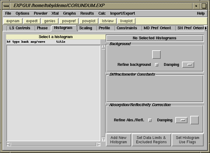
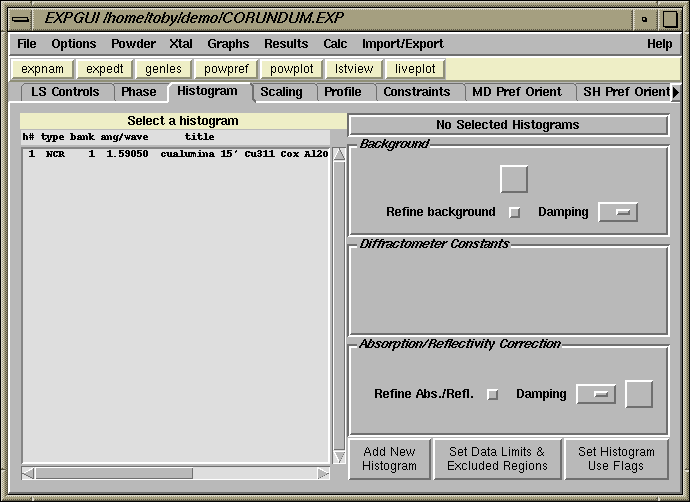
The Histogram panel is selected by clicking on the Histogram tab, as is shown
below. In this case, no data has been defined, as can be determined
by the absence of entries in the histogram selection box, in the upper left.
The "Add New Histogram" button, at the lower right, is used to add [additional]
powder diffraction data sets to the refinement, as will be demonstrated in this
page. The histogram panel is used
to modify various parameters associated with
each set of diffraction data, for example the diffractometer constants
(such as wavelength), the background function and terms.
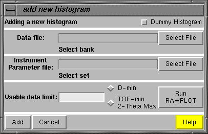 Pressing the "Add New Histogram" button causes the "add new histogram"
window, shown to the right, to be displayed. The entries on this
window are usually considered from top to bottom. The "Dummy Histogram"
option is used to simulate powder diffraction data, and is not
used in this tutorial example. So the next item of interest is to select a
data file. This is done by pressing the upper of the two "Select File"
buttons.
Pressing the "Add New Histogram" button causes the "add new histogram"
window, shown to the right, to be displayed. The entries on this
window are usually considered from top to bottom. The "Dummy Histogram"
option is used to simulate powder diffraction data, and is not
used in this tutorial example. So the next item of interest is to select a
data file. This is done by pressing the upper of the two "Select File"
buttons.
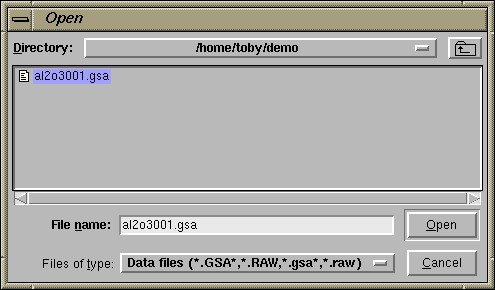 Pressing the "Select File" button creates a file open window, such as
the one to the right (or slightly different in appearance in windows).
Select the input file for this exercise, the file you
downloaded earlier, al2o3001.gsa.
Double-click on the entry, or select is and press the "Open" button.
This open window will then close.
Pressing the "Select File" button creates a file open window, such as
the one to the right (or slightly different in appearance in windows).
Select the input file for this exercise, the file you
downloaded earlier, al2o3001.gsa.
Double-click on the entry, or select is and press the "Open" button.
This open window will then close.
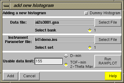 Selecting the raw data file in the open window causes the al2o3001.gsa file
to be loaded into the upper box on the "add new histogram" window. This
file is scanned to and check mark entries are created for each bank
in the file. The al2o3001.gsa file also defines a default instrument
parameter file, which is the bt1demo.ins that was
downloaded earlier, so this file name is
entered into the "Instrument Parameter File" section.
Selecting the raw data file in the open window causes the al2o3001.gsa file
to be loaded into the upper box on the "add new histogram" window. This
file is scanned to and check mark entries are created for each bank
in the file. The al2o3001.gsa file also defines a default instrument
parameter file, which is the bt1demo.ins that was
downloaded earlier, so this file name is
entered into the "Instrument Parameter File" section.
The "Usable data limit" sets the maximum range of data to be used in fitting.
This is usually determined by plotting the data to see where no further
peaks are present. This can be done here with the GSAS RAWPLOT program.
For this exercise, change the defaulted value (the entire data range) to 155
degrees, to exclude a single very broad high-angle peak.
The press the "Add" button in the lower left.
After the "Add" button is pressed, the EXPGUI program runs a GSAS program,
EXPTOOL, that actually adds the data reference to the experiment. If an error
occurs, this result is shown. If no error occurs, the histogram panel
is redisplayed, but this time a histogram appears in the upper left, as
seen below.
Previous:
Adding a Phase
Next step:
Change Background Function