Keywords: reflectivity, neutron, x-ray, spreadsheet, fitting, Solver, GRG2, Parratt formalism.

Abstract

Specular reflectivity experiments have been very successful in the depth profiling of various materials. The inversion problem requires, in general, model fitting. Fitting programs for reflectivity are available at research institutions operating reflectometers, or with commercial instruments. The existing software for reflectivity fitting has proven to be very successful for layered model profiles, however, these programs can be cumbersome in their command structure. Additionally, they do not offer easy use of generic functions (e.g. parabolic profiles) as model profile inputs. Here we attempt to overcome these difficulties by utilizing the advantages of a commonly available spreadsheet as the host environment for fitting. SERF (Spreadsheet Environment Reflectivity Fitting) is comprised of "add-in" functions capable of calculating realistic reflectivity profiles from model scattering length density profiles. The spreadsheet environment offers simultaneous display of numeric and graphical data, and automatic calculation and graph updates when a parameter is changed. These features improve the efficiency of data fitting. Additionally, and most significantly, this method allows flexibility in the profile shapes which can be inputted. The ability to input model profiles, with specific functional forms, simply, may lead to better understanding of data obtained from reflectivity experiments.
 

Introduction
 
Specular reflectivity is a powerful depth profiling technique for a variety of materials. By monitoring the ratio of reflected to incident intensity, R, as a function of the perpendicular component of the wavevector, q_z (inverse length), information about the depth profile in a sample can be obtained. Variation in q_z, is achieved either by variation in the angle of incidence and reflection (monochromatic source), or by changing the wavelength (time of flight source). Contrast is imparted by differences in neutron scattering length density for neutron sources or electron density for x-ray sources. This contrast produces oscillations in the reflectivity data, characteristic of composition depth profile in the sample. Detailed treatments of the technique can be found in the literature.[1-3] The technique offers very high resolution, down as small as a few angstroms, with depth penetrations of several thousand angstroms. Typically there is nominal beam damage to the sample, allowing sequential analysis of a single sample after various treatments. Reflectivity versus wavevector data do not include phase information, and therefore can not be directly inverted to composition versus depth, except in a few special cases.[3]  Consequently, this inversion must be accomplished via model fitting. In this work we have worked to improve the speed and flexibility of the tools used to perform these fitting operations, hopefully further extending the usefulness of the reflectivity technique.

 
Fitting programs for reflectivity are available at research institutions operating reflectometers, or commercially with the instruments themselves. The fitting programs from the NIST Cold Neutron Research Facility (CNRF), with which these authors are familiar with, are either Unix or DOS based, and have proven to be very successful in fitting layered structures. Despite this success, these programs have a relatively cumbersome command structure, and do not offer flexibility in the model profile shapes allowed as inputs. By developing "add-in" functions capable of calculating realistic reflectivity profiles from model scattering length depth profiles within a commonly available spreadsheet (Microsoft Excel^®) performance is improved. The spreadsheet environment offers simultaneous display of numeric and graphical data, as well as automatic calculation and graph update upon the change of a parameter. An additional advantage is the ability to simply input specific functional forms for the scattering length density profile. The following will detail the methods used to calculate profiles and give examples of SERF (Spreadsheet Environment Reflectivity Fitting).
 

Method

The general approach used herein is to utilize the spreadsheet as a powerful front end for a series of add-in functions which calculate reflectivity profiles. All of the functions described are Fortran 90 based. The compilation is done such that the spreadsheet program can call the executable code, similar to commonly used functions like "slope" that are packaged with commercial spreadsheets. All information is passed from the spreadsheet to Fortran using OLE2 and array formulas, provides efficient data transfer, and rapid calculation, even for complicated models. Reflectivity is calculated using the formalism developed by Parratt,[4] with the addition of absorption terms. This approach takes input as layer thickness, d(Å), scattering length (or electron) density, r_b (Å^-2), and adsorption coefficient over wavelength, (m/l), for a series of layers. Any arbitrary scattering length density profile can be input by utilizing a series of thin layers which have scattering length densities defined by some generic function r_b(x). In the study of grafted polymer layers in mixed solvents, the volume fraction of the polymer can be calculated from the alpha model, Equation 1.
 

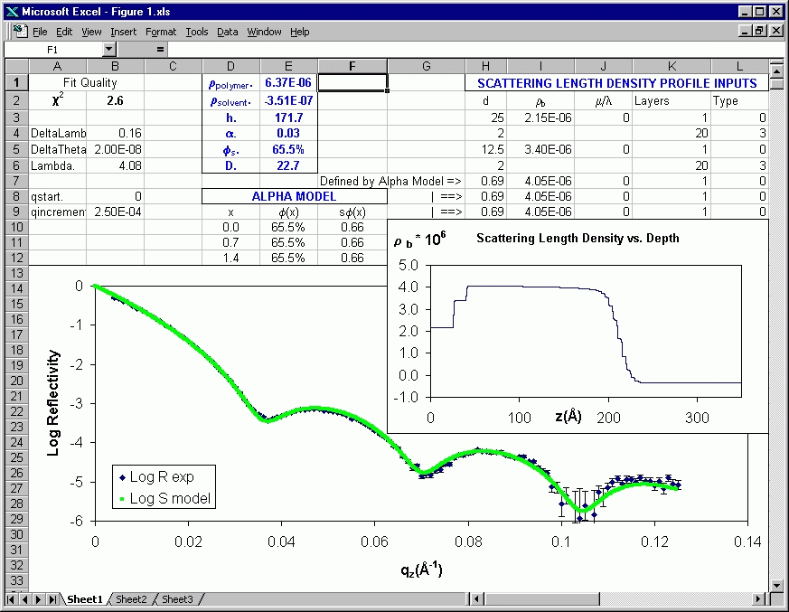
                                                (1)

Figure 1 demonstrates the use of SERF to calculate reflectivity using Equation 1 as an input model. The polymer volume fraction, Equation 1, is calculated in columns D through F, below row 8. The third column, F,  performs a Gaussian smearing on the alpha profile. Column F is then used to define the scattering length profile inputs in column I. This profile is then used to generate a model reflectivity, and compared to experimental data for a deuterated poly(styrene) grafted layer in 75:25 methanol cyclohexane, Figure 1. The width of the smearing function, D., the height of the brush, h., alpha, a., and the volume fraction of polymer at the silicon surface, f_s, are used as adjustable parameters in fitting. To account for instrumental smearing effects the bare reflectivity is treated with a Gaussian smearing function.[5] This smeared reflectivity, as well as the experimental data, are plotted as Log Reflectivity vs. q_z, in Figure 1.

 
Additionally, traditional gradient layers (roughness) with linear, tanh, or erf functional forms have been coded for convenience in the profile interpretation functions. 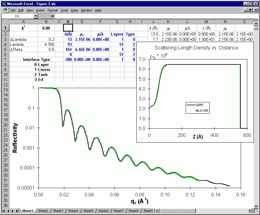Gradient layers are calculated by value matching to the two adjacent plateau layers (type 0), uniformly sectioning the change in scattering length density, and calculating the layer thickness based on the functional form (type 1,2,3), thickness of the gradient region (d(Å)), and the number of steps which discretize the gradient region (layers), all of which are user inputs. Figure 2 shows a simple profile setup using these gradient layers, for a 500Å deuterated poly(styrene) layer on silicon, with beam impinging from air side. As discussed above, the user assigns the thickness of the gradient regions. The assignment of this thickness does not affect the thickness of the adjacent layers, unlike other fitting programs, which create gradient regions by subtracting equally from the adjacent layers. This allows the user to account for nonuniform effects of roughness on the two adjacent layers. Additionally, "Data" in Figure 2 has been calculated using the same model parameters (except for roughness due to the difference in definition discussed above) and imported to the spreadsheet from a fitting program used at NIST, mlayer^©, as a check of these functions. Chi-squared, c² , the sum of the squared differences between SERF and mlayer^© values, divided by a small error allowance, is less than 1, indicating the excellent fit, which can also be seen in the plot of Reflectivity versus q_z. Similar qualification has been performed for air and silicon side measurements for bare reflectivity without roughness, smeared reflectivity without roughness, rough layers without smearing, and finally the combination of all functions, as seen in Figure 2.
 

Figure 2: Screen shot from Microsoft Excel^® demonstrating the ability of SERF in handling traditional layer profiles. Data are taken from a proven fitting program, mlayer^©, and are indicated in green. The inputs to SERF are indicated in blue, outputs are plotted as scattering length density vs. distance and Reflectivity vs. q_z(Å^-1). The excellent "fit" is indicative of identical predictions from SERF and mlayer^©.
 

Fitting is accomplished using the Solver routine packaged with Microsoft Excel^®. Solver is a powerful nonlinear least squares fitting routine. It allows minimization of any function, defined within a spreadsheet cell, by changing any number of parameters. A common example is minimization of c² in Figure 2, by changing the thickness of the gradient and bulk layers. Each of these parameters can also be subjected to constraints, a feature not allowed in some programs. The solver routine is based on the GRG method[6-7], and has been developed by Frontline Systems.[9]
 

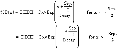
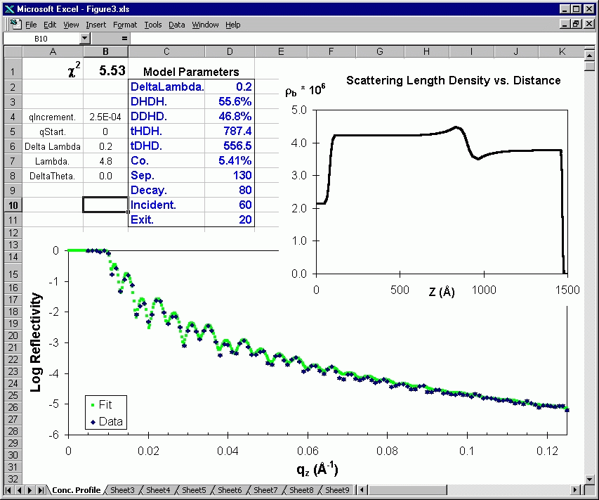
Welp, et al. [8] have used these functions for fitting neutron reflectivity data for a very specialized experiment which directly probes the dynamics of a polymer chains at a polymer-polymer interface in the melt. The samples are composed of two layers of triblock poly(styrene) which are each ~50% deuterated. They differ in the section of the chain that is deuterated. Because of the triblock labeling, the scattering length profiles expected in these samples are complex. Figure 3 shows the profile used and a representative fit to a data file, obtained at NIST CNRF. The profile is composed of two decaying exponential terms determining the deuterium fraction in a given thin layer, Equation 2, and three error function gradient regions.

                                        (2)

The incident medium is silicon, indicated at the left of the scattering length density vs. depth profile, and the final layer is air, at the extreme right. The variables in the model are noted in blue in Figure 3, and include the composition of the two polymer layers, DHDH. and DDHD., excess concentration caused by interdiffusion, Co., decay constant of the exponential terms, Decay., and thickness of the three gradient layers, IncidentRough., Sep., and ExitRough., for the Si/polymer, polymer/polymer, and polymer/air interfaces, respectively. These fitting tools were essential for this research as they allowed calculation of reflectivity from this complex profile that could be readily inputted. The ability to alter any of the parameters shown in boldface print in Figure 3, and see immediate update of the fit quality, both graphically and numerically, has provided much information as to the sensitivity of the fit to the various parameters.
 

Figure 3: Screen shot from Microsoft Excel^® demonstrating the use of SERF for polymer interdiffusion experiments with complex scattering length density profiles. The deuterium concentration profile is a function of parameters, in blue, and given by Equation 2. The scattering length density profile plot is derived from the deuterium depth profile by a SERF function. Model reflectivity, in green, is calculated and plotted along with experimental data as Log Reflectivity vs. q_z(Å^-1).
 

Conclusion

This paper has briefly listed the approach and capabilities of a new series of fitting tools for reflectivity data. This approach has proven to be more user friendly than other approaches. It allows complete flexibility in the type of profiles that can be inputted. Additionally, once a profile has been defined in terms of a few parameters, immediate recalculation and update of all figures follow a change to any of the parameters. This gives the user an immediate feel for the effect of a given parameter on the model profile without cumbersome commands required to display data in other implementations.
 
Additional information, instructions, and free download of all functions are available at http://www.kalergroup.che.udel.edu/KalergroupWebPage/Software/SoftwareIndex.htm
 

Acknowledgments

Funding support for K.A.Welp from NSF, grant DMR-9596-267, and for C. Co from NSERC (National Science and Engineering Research Council of Canada). K.A.W. would like to thank support from the Delaware Space Grant College Fellowship Program. The authors would also like to acknowledge the help and advice of S. K. Satija.
 

References
 

1. Russell, T.P. Materials Science Reports, 1990, 5, 171.
2. Lekner, J.L. Theory of Reflection; Martinus Nijhoff Publishers: Dodrecht, 1987.
3. Stamm, M. In Physics of Polymer Surfaces and Interfaces; Sanchez, I.C. Ed; Butterworth-Heinemann: Boston, 1992, pp 163-201.
4. Parratt, L.G. Phys. Rev., 1954, 95, 359.
5. Hamley, I.W.; Pedersen, J.S.; J. Appl. Cryst., 1994, 27, 29; 36.
6. Lasdon, L.S.; Waren, A.; Jain, A.; Ratner, M. ACM Transactions on Mathematical Software, 1978, 4, 34.
7. Lasdon, L.S. and Smith, S. ORSA Journal on Computing 1992, 4, 2.
8. Welp, K.A.; Wool, R.P., Satija, S.K., Mays, J.M. Mays; Pispas, S.; submitted to Macromolecules.
9. www.frontsys.com.